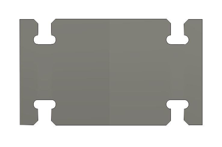
GIK Geometry Design Exploration
To design the most effective GIK part, there are a number of factors to consider. We will look at parameters such as thickness, length, and height. These parameters can be expressed as a function of lattice pitch, which allows us to compare them on the same plot and see what effect they have on the metrics we aim to maximize: functional length and functional density.
import numpy as np
from scipy import integrate
from matplotlib import pyplot as plt
import matplotlib.patches as mpatches
import matplotlib.lines as mlines

# Magic function to make matplotlib inline; other style specs must come AFTER
%matplotlib inline
%config InlineBackend.figure_formats = {'png', 'retina'}
# %config InlineBackend.figure_formats = {'svg',}
plt.ioff()    # this stops the graphs from overwriting each other
Thickness
This parameter is governed by commonly available sheet thicknesses. We need a stiff insulator insulator thinner than our final thickness for many functional part-types. Garolite is a good material for this but is only available in thicknesses down to 5mil. This means that 10mil is reasonable for the overall part thickness.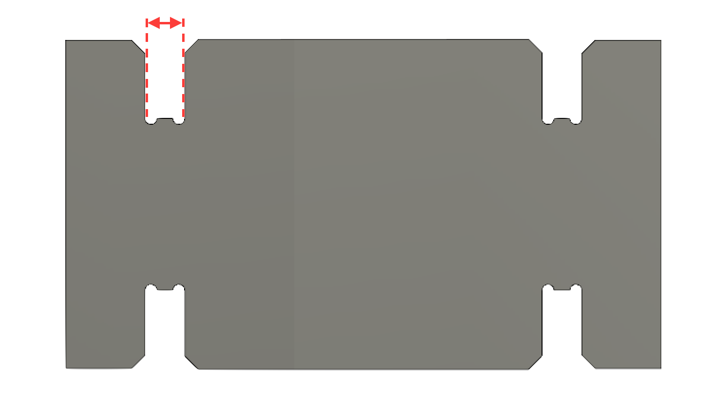
thickness = 0.254
Pitch
We'll use pitch as our independent variable and define it in terms of multiples of the thickness.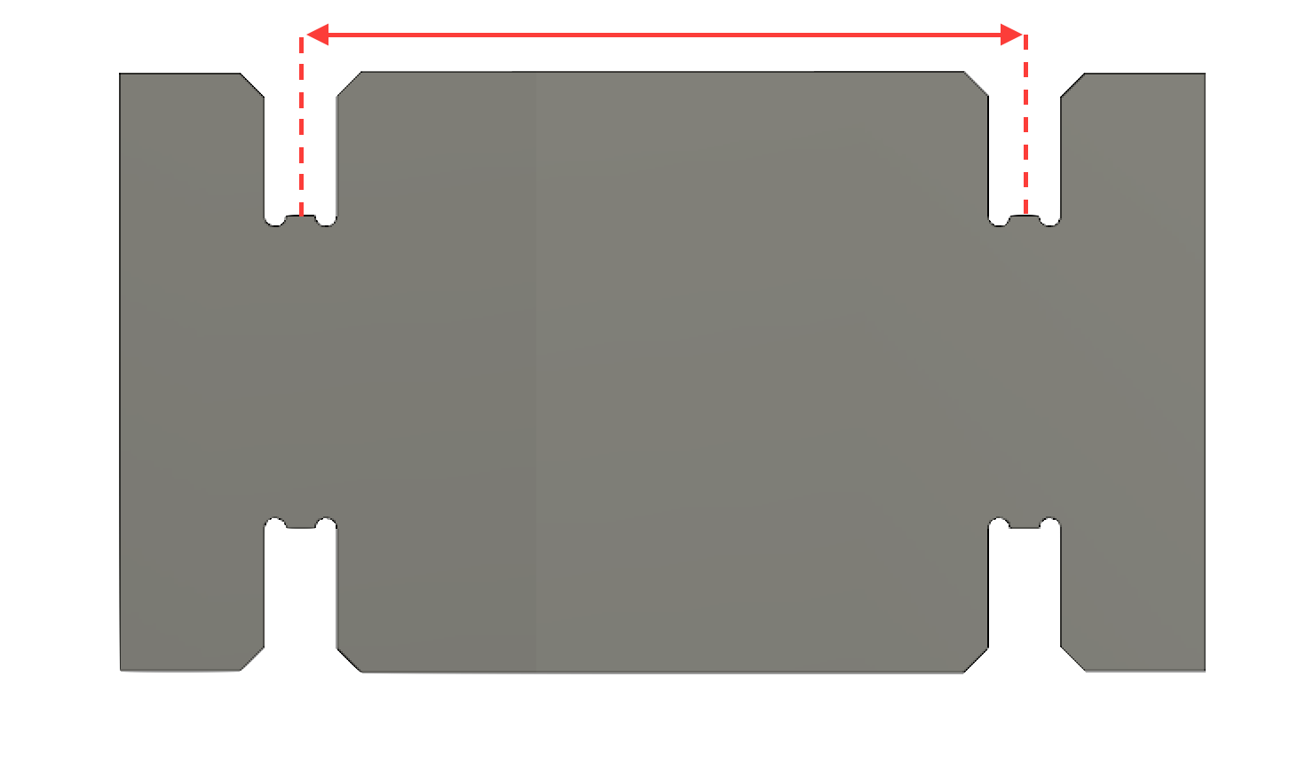
minx = 2*thickness
maxx = 20*thickness
pitch = np.arange(minx,maxx,thickness/5)
Aspect Ratio
We impose an aspect ratio constraint such that the part is longer than it is tall. This is helpful because of the vertically-assembled nature of the lattice. This sets a maximum constraint on the height of the part, such that: $$ height <= \frac{FL}{1.25} $$where $FL$, or functional length, is the interior length of the part that can be used to house functional elements and is defined as:
$$ FL = pitch-thickness $$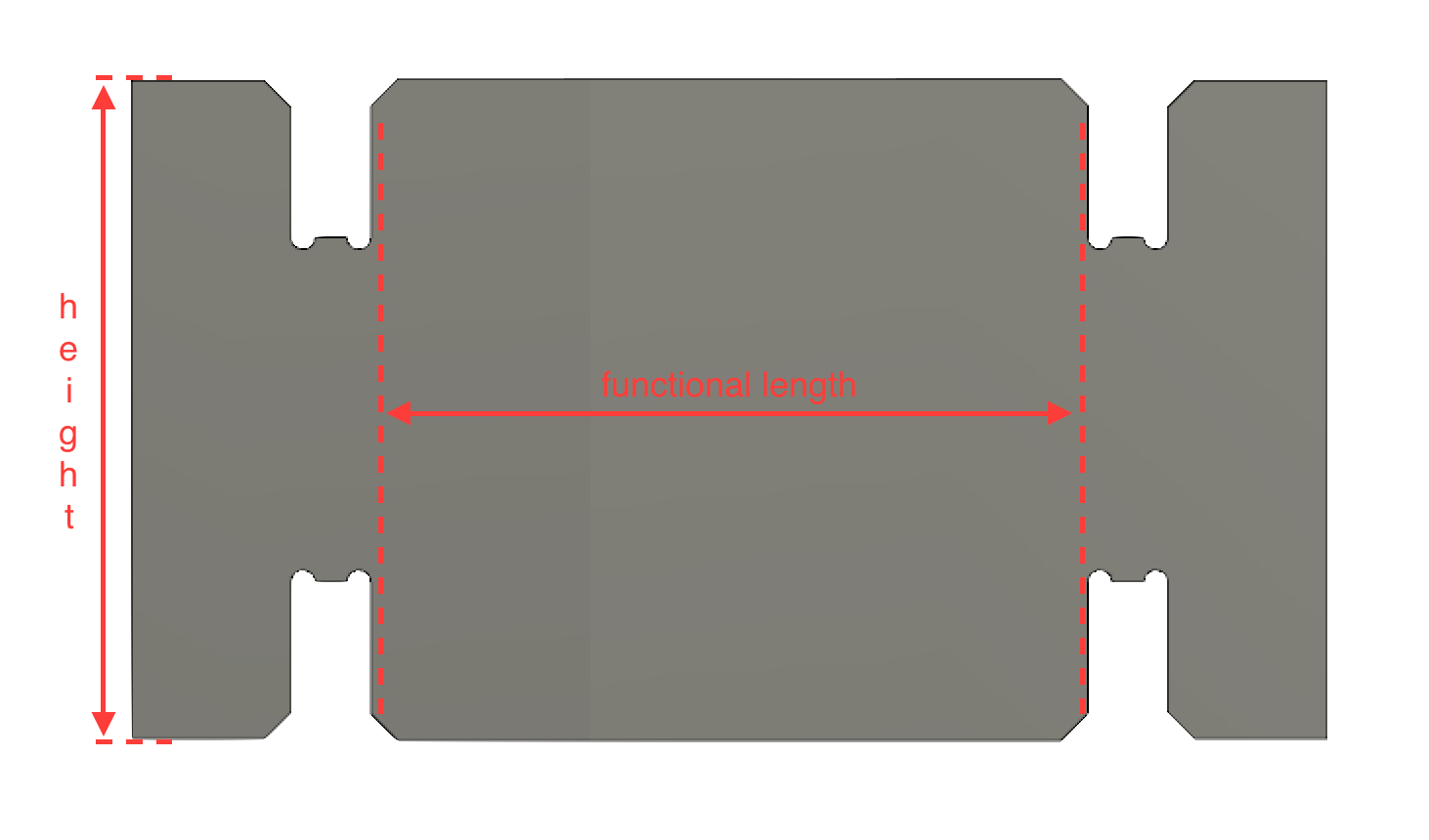
# Funcitonal Length
FL = pitch-thickness

# Aspect Ratio
height_1 = FL / 1.125
Manufacturability – Height
Additional constraints are imposed by our choice of manufacturing method. If we want to be able to make these using the wire-edm, there's a constraint imposed by the kerf of the cut. Using the standard 0.006" wire cuts with a 0.010" kerf. This kerf imposes a constraint on the slot depth, which in turn, is linked to the height of the part. Therefore, this sets a minimum value for the height. $$ SD = \frac{height}{4.2} $$ $$ SD >= 2\times kerf $$ $$ \therefore \ \ height >= 4.2 \times 2 \times kerf $$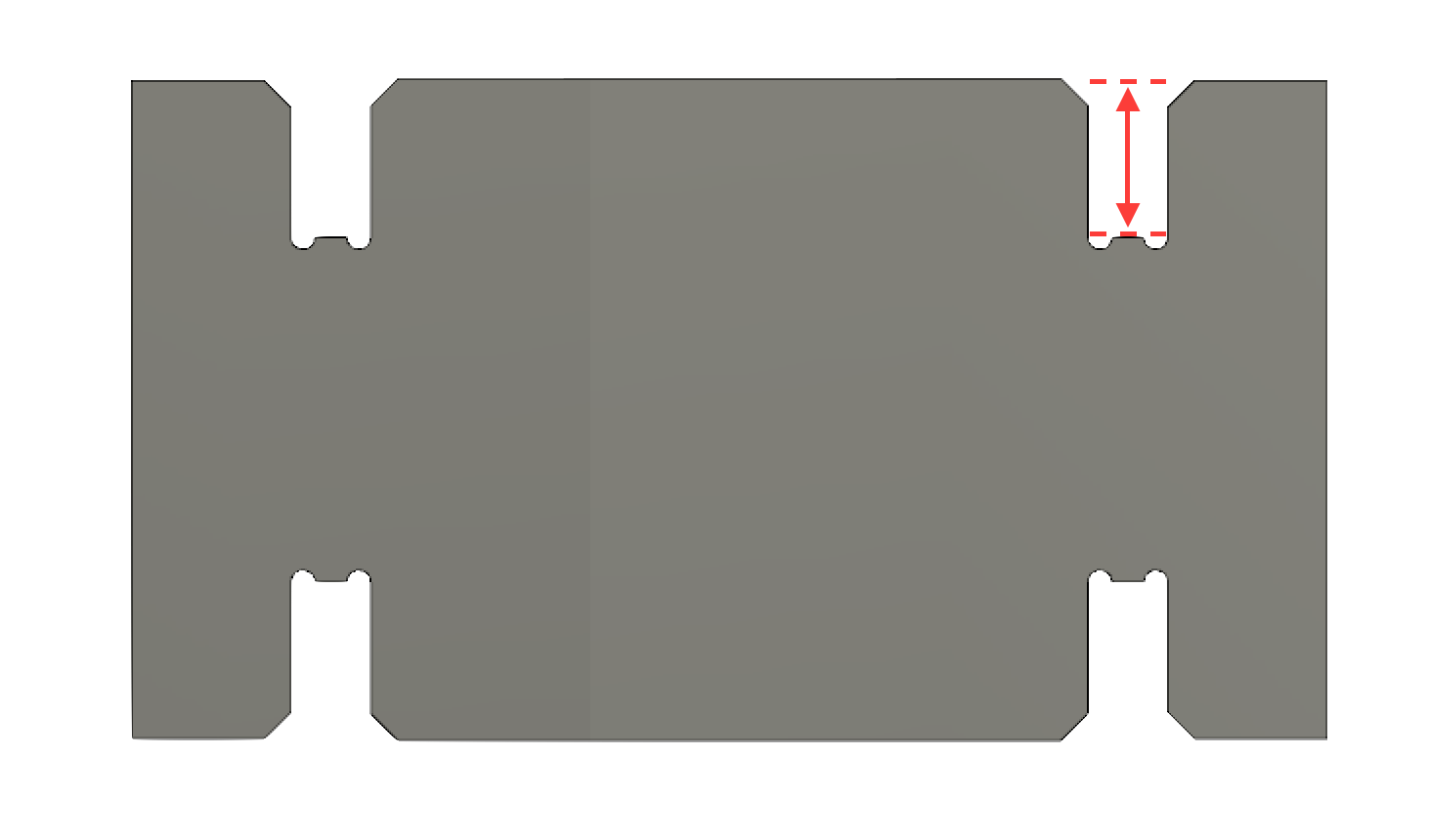
# Wire EDM Manufacturability
kerf = 0.254
height_2 = np.ones(len(pitch))*4.2*3*kerf
Given both a minimum bound and maximum bound for the height, we can plot both and define a region for valid designs.
# Setup Plotting
colors = ['#0571b0','#92c5de','#f4a582','#ca0020']
fig, ax1 = plt.subplots()

font = {'family' : 'Bitstream Vera Sans',
        'weight' : 'normal',
        'size'   : 14}

plt.rc('font', **font)

min_height, = ax1.plot(pitch,height_1,colors[0],lw=1.2,label="Height")
max_height, = ax1.plot(pitch,height_2,colors[1],lw=1.2)
ax1.fill_between(pitch, height_1, height_2, where=((height_1>=height_2)), interpolate=True, facecolor='#4393c3', alpha=0.25)

ax1.set_xlabel('Pitch [mm]',fontsize=18)
ax1.set_ylabel('Dimension [mm]',fontsize=18)

# set Y-scale for only ax1
plt.ylim(0,10)
# set X-scale for both axes
plt.xlim(minx,maxx-0.1)
fig.set_size_inches(16, 12,forward=True)

# Legend
blue_patch = mpatches.Patch(color='#4393c3', alpha=0.5, label='Height Constraints')
ax1.legend(loc='upper left',handles=[blue_patch])
fig

Manufacturability – Length
The kerf of the manufacturing process also imposes constraints on the length of the part. Because we want the slot to be sufficiently stiff, there should be plenty of room between the distal slot face and the end of the part to allow for dogbones in the interior corners or the slots. We can define the following heuristic which sets a minimum on the part length: $$ \frac{(length - pitch - thickness)}{2} >= 3 \times kerf$$$$ \therefore \ \ length >= 3 \times kerf + 2 \times thickness + pitch$$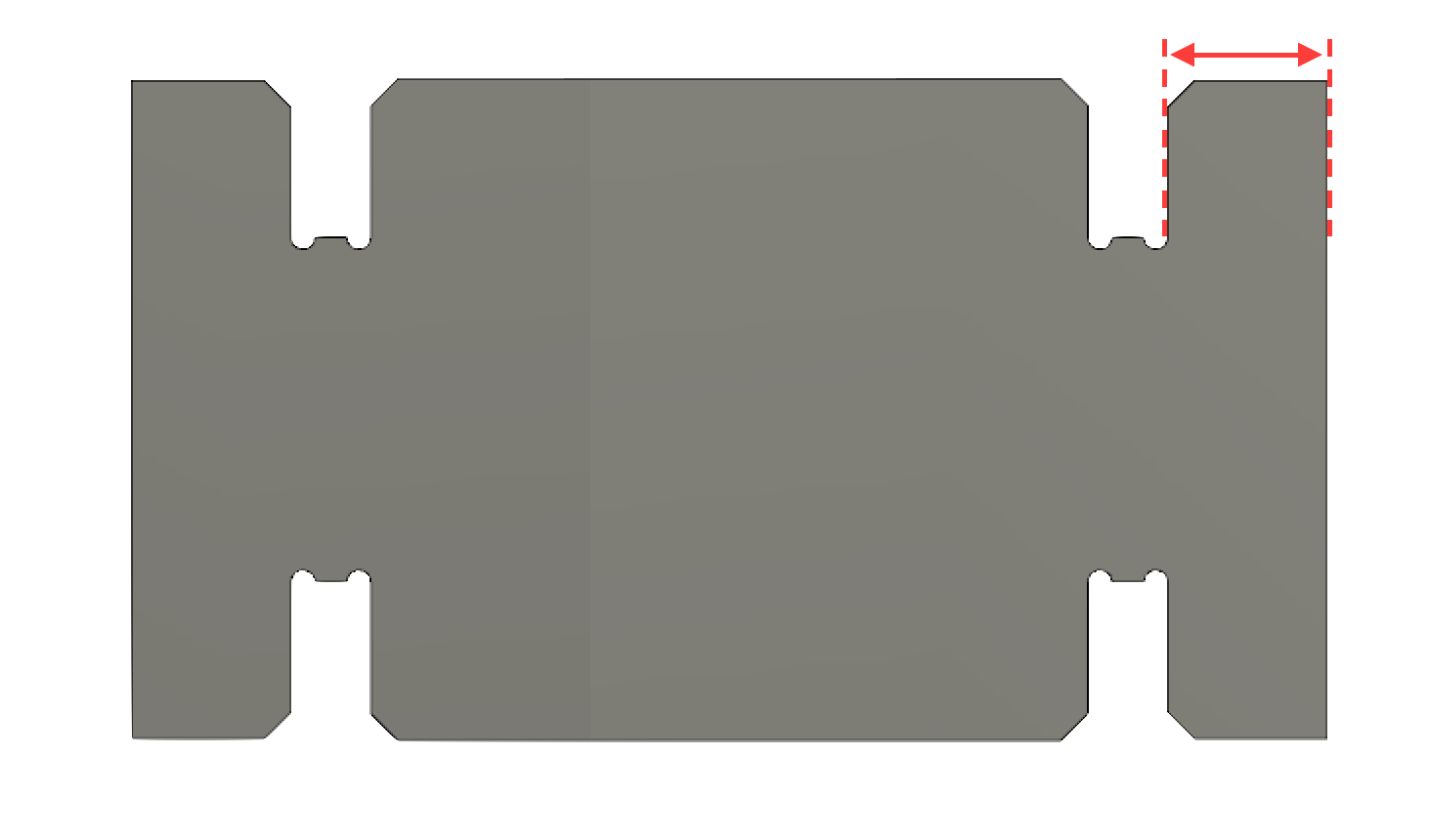
length_1 = 2.5*kerf + 2*thickness + pitch
Lattice Constraints
The length of the part is constrained by the geometry of the lattice such that it can be no longer than twice the pitch. Which is to say, the maximum length is: $$ length < 2 \times pitch $$# Max Length
length_2 = 2*pitch
Given these length constraints, we can add them to the plot:
min_length, = ax1.plot(pitch,length_1,colors[2],lw=1.2,label="Length")
max_length, = ax1.plot(pitch,length_2,colors[3],lw=1.2)
ax1.fill_between(pitch, length_1, length_2, where=length_1<=length_2, interpolate=True, facecolor='#d6604d', alpha=0.25)

red_patch = mpatches.Patch(color='#d6604d', alpha=0.5, label='Length Constraints')
ax1.legend(loc='upper left',handles=[blue_patch,red_patch])

# Increase font size for legibility
for item in ([ax1.title, ax1.xaxis.label, ax1.yaxis.label] +
         ax1.get_xticklabels() + ax1.get_yticklabels()):
	item.set_fontsize(18)
fig

Optimizing the Parts – Functional Length
These constraints provide regions within which we can choose part designs, but they don't say anything about what an optimal part design is.The first metric we look to optimize is the functional length. A good part design will maximize the functional region of the part with respect to its overall size. We can define a normalized functional length as:
$$ \hat{FL} = \frac{FL}{length} $$For the purposes of this plot, we'll use the minimum bound on length since this results in maximizing the normalized functional length.
# Normalized Functional Length
norm_FL = FL/length_1
Optimizing the Lattice – Functional Density
Another competing metric we can look at is the functional density of the lattice. This is the proportion of the lattice volume which is able to contain functionality. We can define it as: $$ \hat{FD} = \frac{n\_parts \times FL \times height \times thickness}{(n\_pitches^2) \times pitch \times pitch \times height} $$where $n\_parts$ is the number of parts in a $n\_pitches$ by $n\_pitches$ section of the lattice.
# Functional Density
FD = FL*thickness*18 /(9*pitch*pitch)
We can add these quantities to the plot:
# Setup Plotting 3
colors = ['#0571b0','#92c5de','#f4a582','#ca0020']
fig, ax1 = plt.subplots()

font = {'family' : 'Bitstream Vera Sans',
        'weight' : 'normal',
        'size'   : 14}

plt.rc('font', **font)

min_height, = ax1.plot(pitch,height_1,colors[0],lw=1.2,label="Height")
max_height, = ax1.plot(pitch,height_2,colors[1],lw=1.2)
ax1.fill_between(pitch, height_1, height_2, where=((height_1>=height_2)), interpolate=True, facecolor='#4393c3', alpha=0.25)

min_length, = ax1.plot(pitch,length_1,colors[2],lw=1.2,label="Length")
max_length, = ax1.plot(pitch,length_2,colors[3],lw=1.2)
ax1.fill_between(pitch, length_1, length_2, where=length_1<=length_2, interpolate=True, facecolor='#d6604d', alpha=0.25)

ax1.set_xlabel('Pitch [mm]',fontsize=18)
ax1.set_ylabel('Dimension [mm]',fontsize=18)

# set Y-scale for only ax1
plt.ylim(0,10)

# Setup Second Axis
ax2 = ax1.twinx()
func_len, = ax2.plot(pitch,FL/length_1,'#4daf4a',lw=2)
func_den, = ax2.plot(pitch,FD,'#984ea3',lw=2)
# both, = ax2.plot(pitch,FD+FL/length_1,'#984ea3',lw=2)
ax2.set_ylabel('Normalized Value',fontsize=18,color='#d7191c')

# Legend
red_patch = mpatches.Patch(color='#d6604d', alpha=0.5, label='Length Constraints')
blue_patch = mpatches.Patch(color='#4393c3', alpha=0.5, label='Height Constraints')
green_line = mlines.Line2D([], [],lw=3, color='#4daf4a', label='Normalized Functional Length')
purple_line = mlines.Line2D([], [],lw=3, color='#984ea3', label='Normalized Functional Density')
ax2.legend(loc='upper left',handles=[red_patch, blue_patch, green_line, purple_line])

# set X-scale for both axes
plt.xlim(minx,maxx-0.1)

# set figure size
fig.set_size_inches(16, 12,forward=True)

# Recolor right-side Y-axis and corresponding legend handles
ltext = plt.gca().get_legend().get_texts()
plt.setp(ltext[2], color='#d7191c')
plt.setp(ltext[3], color='#d7191c')
for t1 in ax2.get_yticklabels():
	t1.set_color('#d7191c')

# Increase font size for legibility
for item in ([ax1.title, ax1.xaxis.label, ax1.yaxis.label] +
         ax1.get_xticklabels() + ax1.get_yticklabels()):
	item.set_fontsize(18)

for item in ([ax2.title, ax2.xaxis.label, ax2.yaxis.label] +
     ax2.get_xticklabels() + ax2.get_yticklabels()):
	item.set_fontsize(18)

fig

Clearly the two quantities we want to maximize are in opposition with each other but a reasonable choice might be somewhere at the extents of the manufacturing constraints.
Interestingly, it turns out that the "classic" GIK is exactly at this point...
from matplotlib._png import read_png
from matplotlib.cbook import get_sample_data
from matplotlib.offsetbox import TextArea, DrawingArea, OffsetImage, \
    AnnotationBbox

ax1.axvline(x=3.81,linestyle='dashed',color='k')
classic_l, = ax1.plot(3.81,4.953,'ko',markersize=8,label='Classic GIK')
classic_h, = ax1.plot(3.81,3.175,'ko',markersize=8)

ax2.legend(loc='upper left',handles=[red_patch, blue_patch, green_line, purple_line,classic_l])

fn = get_sample_data("files/classic_gik.png", asfileobj=False)
arr_lena = read_png(fn)

imagebox = OffsetImage(arr_lena, zoom=0.25)
xy = (4.25,.525)
ab = AnnotationBbox(imagebox, xy,
                    xybox=(3.5, 6),
                    xycoords='data',
                    boxcoords="offset points",
                    pad=0.25,
                    arrowprops=dict(arrowstyle="->",
                                    connectionstyle="angle,angleA=0,angleB=90,rad=3")
                    )

ax2.add_artist(ab)

fig

Adjusting Our Manufacturing Constraints
This plot shows that our ability to manufacture these parts at smaller scales is currently limited by the kerf of the Wire-EDM process.The the 0.002" is too impractical for mass-production of these parts, it's possible 0.004" wire could be a happy medium between the two wire sizes we currently use.
# Effect of Thinner Wire
kerf = .007*25.4
height_2 = np.ones(len(pitch))*4.2*2*kerf
length_1 = 2.5*kerf + 2*thickness + pitch
We can look at how the design space is opened up by reducing the kerf.
# Setup Plotting 4
colors = ['#0571b0','#92c5de','#f4a582','#ca0020']
fig, ax1 = plt.subplots()

font = {'family' : 'Bitstream Vera Sans',
        'weight' : 'normal',
        'size'   : 14}

plt.rc('font', **font)

min_height, = ax1.plot(pitch,height_1,colors[0],lw=1.2,label="Height")
max_height, = ax1.plot(pitch,height_2,colors[1],lw=1.2)
ax1.fill_between(pitch, height_1, height_2,
                 where=((height_1>=height_2)), interpolate=True,
                 facecolor='#4393c3', alpha=0.25)

min_length, = ax1.plot(pitch,length_1,colors[2],lw=1.2,label="Length")
max_length, = ax1.plot(pitch,length_2,colors[3],lw=1.2)
ax1.fill_between(pitch, length_1, length_2,
                 where=length_1<=length_2, interpolate=True,
                 facecolor='#d6604d', alpha=0.25)

ax1.set_xlabel('Pitch [mm]',fontsize=18)
ax1.set_ylabel('Dimension [mm]',fontsize=18)

# set Y-scale for only ax1
plt.ylim(0,10)

# Setup Second Axis
ax2 = ax1.twinx()
func_len, = ax2.plot(pitch,FL/length_1,'#4daf4a',lw=2)
func_den, = ax2.plot(pitch,FD,'#984ea3',lw=2)
# both, = ax2.plot(pitch,FD+FL/length_1,'#984ea3',lw=2)
ax2.set_ylabel('Normalized Value',fontsize=18,color='#d7191c')

ax1.axvline(x=3.81,linestyle='dashed',color='k')
ax1.plot(3.81,4.953,'ko',markersize=8,label='classic_l')
ax1.plot(3.81,3.175,'ko',markersize=8)

height_intersect = 2.54

ax1.axvline(x=height_intersect,linestyle='dashed',color='k')
new_gik, = ax1.plot(height_intersect,
                    (height_intersect-thickness)/1.125,'ks',
                    markersize=8,label='New GIK')
ax1.plot(height_intersect,height_intersect+2.5*kerf+2*thickness,'ks',markersize=8)

fn = get_sample_data("files/new_gik.png", asfileobj=False)
arr_lena = read_png(fn)

imagebox = OffsetImage(arr_lena, zoom=0.3)
xy = (2.15,.485)
ab = AnnotationBbox(imagebox, xy,
                    xybox=(3.5, 6),
                    xycoords='data',
                    boxcoords="offset points",
                    pad=0.15,
                    arrowprops=dict(arrowstyle="->",
                                    connectionstyle="angle,angleA=0,angleB=90,rad=3")
                    )

ax2.add_artist(ab)

fn = get_sample_data("files/classic_gik.png", asfileobj=False)
arr_lena = read_png(fn)

imagebox = OffsetImage(arr_lena, zoom=0.25)
xy = (4.2,.525)
ab = AnnotationBbox(imagebox, xy,
                    xybox=(3.5, 6),
                    xycoords='data',
                    boxcoords="offset points",
                    pad=0.25,
                    arrowprops=dict(arrowstyle="->",
                                    connectionstyle="angle,angleA=0,angleB=90,rad=3")
                    )

ax2.add_artist(ab)

ax2.arrow(3.81, .265, -1.27+0.05, 0, head_width=0.01, head_length=0.05, fc='k', ec='k')

# Legend
red_patch = mpatches.Patch(color='#d6604d', alpha=0.5,
                           label='Length Constraints')
blue_patch = mpatches.Patch(color='#4393c3', alpha=0.5,
                            label='Height Constraints')
green_line = mlines.Line2D([], [],lw=3, color='#4daf4a',
                           label='Normalized Functional Length')
purple_line = mlines.Line2D([], [],lw=3, color='#984ea3',
                            label='Normalized Functional Density')
ax2.legend(loc='upper left',
           handles=[red_patch, blue_patch, green_line,
                    purple_line, classic_l, new_gik])

# set X-scale for both axes
plt.xlim(minx,maxx-0.1)

# set figure size
fig.set_size_inches(16, 12,forward=True)

# Recolor right-side Y-axis and corresponding legend handles
ltext = plt.gca().get_legend().get_texts()
plt.setp(ltext[2], color='#d7191c')
plt.setp(ltext[3], color='#d7191c')
for t1 in ax2.get_yticklabels():
	t1.set_color('#d7191c')

# Increase font size for legibility
for item in ([ax1.title, ax1.xaxis.label, ax1.yaxis.label] +
         ax1.get_xticklabels() + ax1.get_yticklabels()):
	item.set_fontsize(18)

for item in ([ax2.title, ax2.xaxis.label, ax2.yaxis.label] +
     ax2.get_xticklabels() + ax2.get_yticklabels()):
	item.set_fontsize(18)

fig

So the final geometry comes out to:
print("thickness: ", thickness)
print("pitch: ", height_intersect)
print("height: ", (height_intersect-thickness)/1.125)
print("length: ", 2.5*kerf + 2*thickness + height_intersect)
print("slot_depth: ", (height_intersect-thickness)/1.125/4.2)